A Deep Dive into KNN

01Introduction

KNN or the K-nearest neighbor is a highly preferred ML algorithm amongst ML practitioners. It is widely used in several business cases such as evaluating academic performance, in diagnostic systems, in wireless sensor networks, search engines and medical diagnosis. We can apply it for both classification and regression predictive problems. When applied to classification, it uses the entire training data and thus may be called a lazy learning algorithm. It does not make any assumptions on the underlying data and thus can be considered being a non-parametric learning algorithm. The algorithm does not require any training before making predictions, and thus new data can be added seamlessly without affecting the prediction accuracy. Considering these benefits, it is worthwhile understanding its implementation. In this tutorial I will show you a very efficient implementation of KNN in Python.

02Illustrative Case Study

To understand the principles of KNN, let us look at some real-life examples.

We categorize the food that we eat into different categories, viz. - fruits, vegetables, grains, proteins, dairy, and so on. For categorization, we distinguish them from each other by many chemical and physical features. For our illustration, we will categorize food using the two simple features, namely crunchiness and sweetness. The following picture shows few food items belonging to different categories classified using these two features.

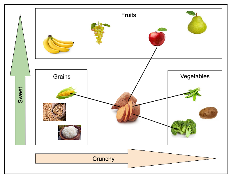
We plot the two properties on x and y axes and do the food items placement without mentioning the actual feature values. We do a bounding rectangle to categorize them into three categories - fruits, vegetables, grains. Now, our aim is to classify a sweet potato to fit into one of these three categories based on the two features - sweet and crunchy. We use the KNN algorithm for this inference. We base our algorithm on the principle of finding the closest neighbours. A closest neighbour is decided by computing the Euclidean distance (I will explain this later) between the two neighbours. The smaller this distance is, more is the similarity between these two items. In our example, the closest items to a sweet potato are apple, green bean, broccoli and corn. Because the vegetable wins the most votes, we assign sweet potato to the class of a vegetable.

This trivial real-life example has given you a brief description of how KNN works. Now we will move into an in-depth treatment on KNN’s theory.

03How KNN Works?

The KNN working is simple, as illustrated in the above example. We compute the Euclidean distance of a test item with all other items and pick up the one with the least distance as our inference. In real-world, the dataset comprises many features and not just the two as in our earlier illustration. Rather, each row in a dataset contains many columns which we use as features during model training. Thus, while determining the proximity between the two rows, we need to compute the Euclidean distance between all these features and then consider the weighted average of all these distances. We will use some threshold while grouping the item based on this weighted average. To determine the proximity, there are several distance measurements used in practice. I will now describe a few.

04Distance Measure

The measurement of distance determines the similarity of two elements. We can use this measure for clustering, that is categorizing or grouping the items. Typically, we use the following measurements in KNN.

• Euclidean
• Manhattan
• A squared euclidean
• Cosine

05Euclidean Distance

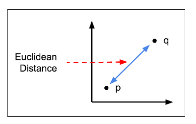
This is the most commonly used measurement in implementing KNN algorithm. We will use this in our implementation. The Euclidean distance is an ordinary straight line between the two points. It is the distance between the points in Euclidean space and we express it mathematically as:

Graphical representation of the euclidean distance is shown below:

06Squared Euclidean Distance

This is identical to the Euclidean distance, except for the square root computation on the entire expression. Mathematically, this is represented as:

07Manhattan Distance

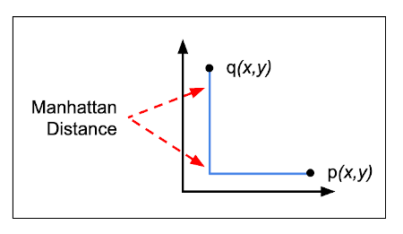
The Manhattan distance is a simple sum of the horizontal and vertical components of the distance between two points. We consider the absolute distance in both directions. Mathematically, it is expressed as:

The graphical representation is shown in the figure below:

08Cosine Distance

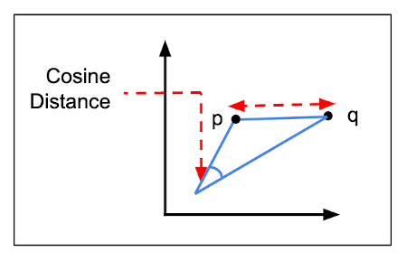
Here, we consider the angle between the two vectors formed by joining the points to the origin. Mathematically, this is expressed as:

The graphical representation is shown in figure below:

With this small introduction to KNN theory, I will now discuss a real-life case study for our KNN implementation.

09Case Study

Breast cancer is one of the most common cancers. An early detection can improve the prognosis and chances of survival significantly. We will implement the KNN algorithm on the dataset of cancer patients to classify the stage of the cancer as malignant or benign. Fortunately for us, the dataset of such cancer patients is available to us as part of the Kaggle competition. The dataset has a vast set of 32 features. So, we will implement the KNN algorithm to compute the Euclidean distance on this vast set of features and take a weighted average to determine the stage of the cancer.

10Creating Project

Create a new Google Colab project and rename it to KNN. If you are new to Colab, then check out this short video

11Importing Libraries

Import the required libraries:

import numpy as np
import pandas as pd    
from random import randrange    
import math    
from math import sqrt    
import operator    
import seaborn as sns    
import matplotlib.pyplot as plt

12Loading Dataset

We take the dataset of this project from the Kaggle site. The dataset shows the breast cancer stage based on the various features of breast mass. The dataset contains 32 features that can predict the stage of breast cancer.

Use the following code to download the dataset into your Colab environment.

!wget https://raw.githubusercontent.com/abcom-mltutorials/knn/main/breast_cancer.csv

Use the read_csv method to load the data as a dataframe

dset = pd.read_csv('breast_cancer.csv')

13Data Preprocessing

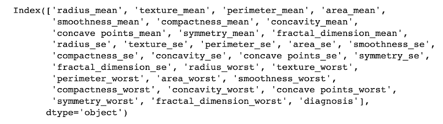
Check the data columns:

dset.columns

The output is shown below:

14Encoding Categorical Columns

Let’s now see the datatypes of all the columns.

dset.dtypes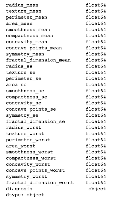

If you examine the data, you notice that the diagnosis column is categorical. We encode it using the following code:

from sklearn import preprocessing
label_encoder = preprocessing.LabelEncoder()      
dset['diagnosis']= label_encoder.fit_transform(dset['diagnosis'])

15Checking Relationships

We generate the heatmap to get the relation between the various features of the dataset. Use the following code for generating heatmap.

corr = dset.corr()
top_corr_features = corr.index      
plt.figure(figsize=(15,15))      
g=sns.heatmap(dset[top_corr_features].corr(),annot=True,cmap="RdYlGn")

The output is shown below:

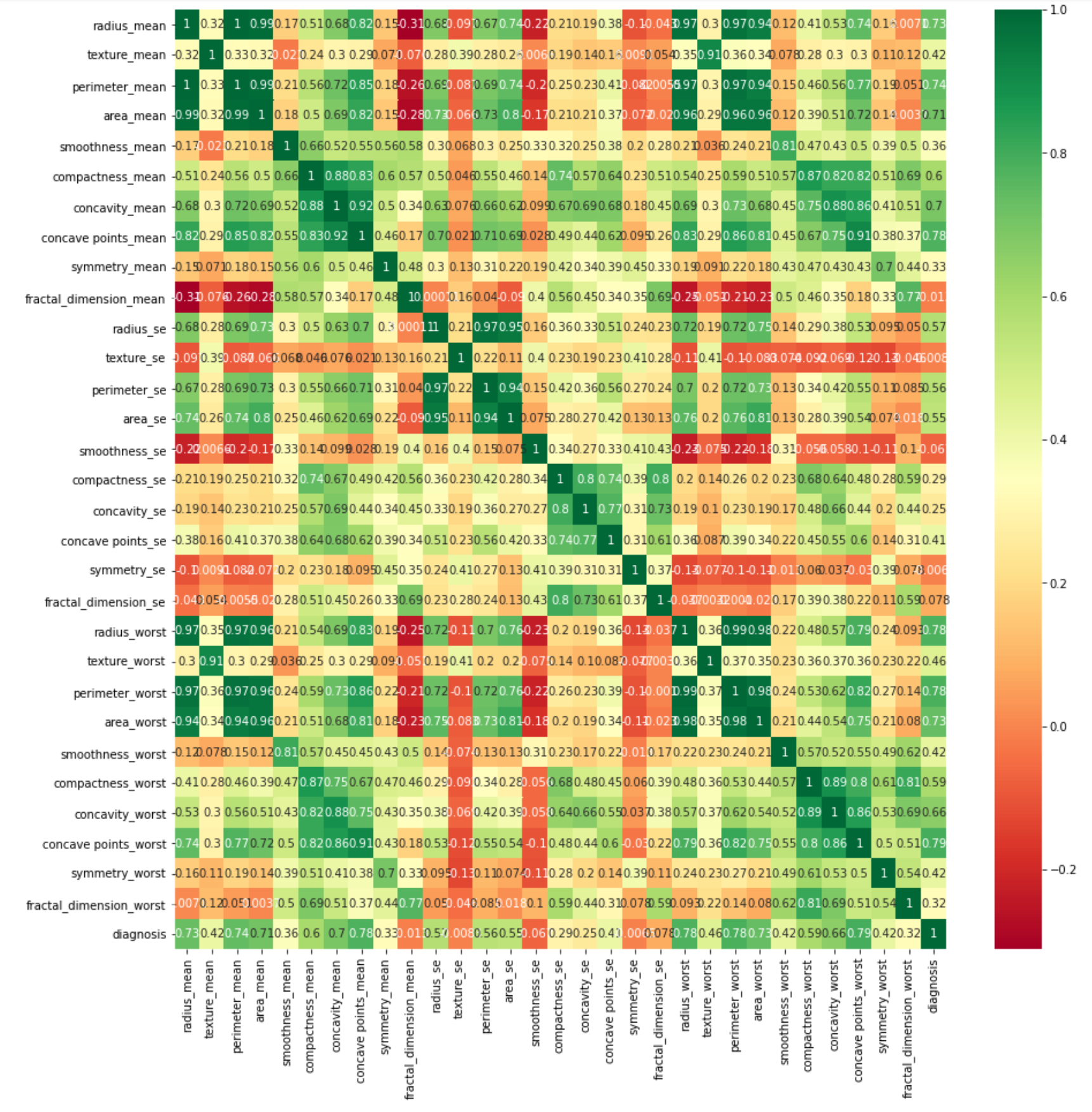
The heatmap shows the numeric percentage of the relationship between any two given features.

16Feature Engineering

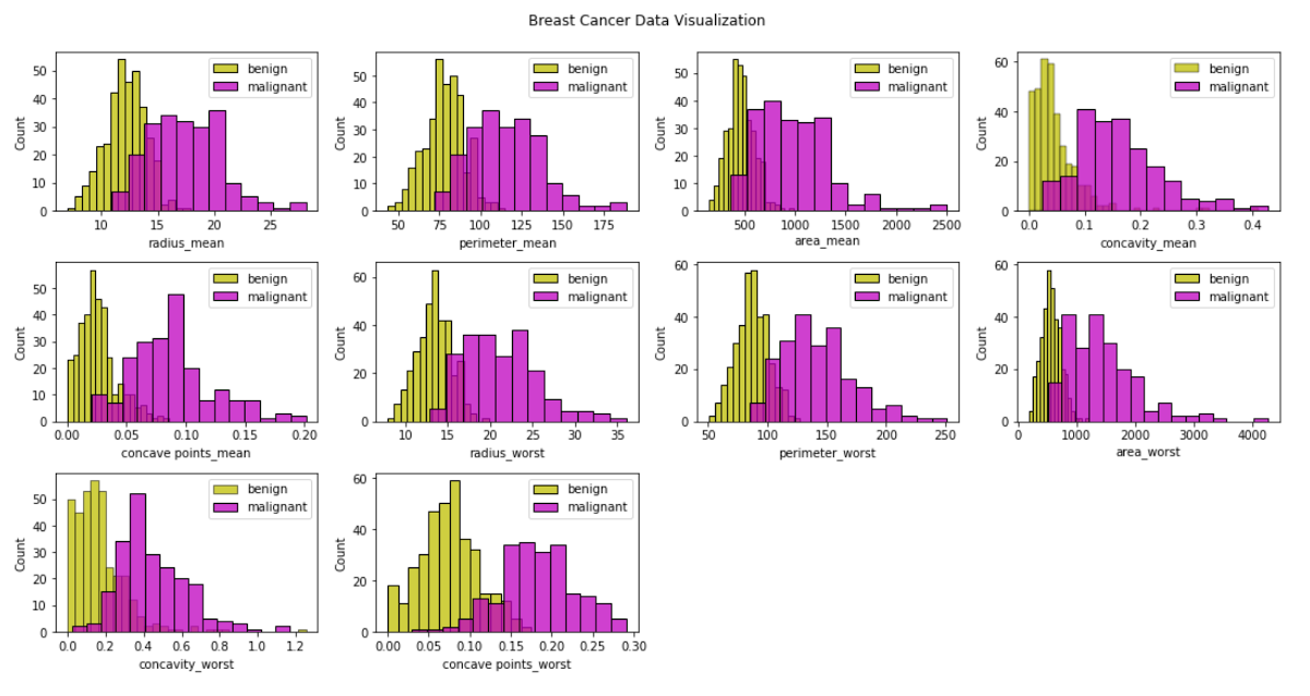
As the dataset contains a very large number of features, we will use some feature engineering technique to reduce the number of features for training. We will develop a function called valuable_features to select the columns which are major contributors in deciding whether the cancer is benign or malignant. We will also use this function to visualize the density of all the selected columns regarding their values, which gives us a region estimate regarding each feature whether the cancer is benign or malignant.

We declare the function:

def valuable_features(dset):

We first generate the correlation matrix:

corr = dset.corr()

Then we get all the columns of our dataset and store it in the columns variable.

columns = np.full((corr.shape[0],), True, dtype=bool)

In the next step we iterate through all the columns of the dataset and compare their correlation with the last column (diagnosis) and remove all columns that have correlation less than 0.6.

for i in range(corr.shape[0]-1):
if corr.iloc[len(dset.columns)-1,i] <= 0.6:      
columns[i] = False

The columns having correlation greater than 0.6 are kept and stored in a variable selected_columns and our dataset is updated to keep only these selected columns.

selected_columns = dset.columns[columns]
dset = dset[selected_columns]

We iterate over all the selected columns excluding the last column (diagnosis) and its length simultaneously using the zip function as shown:

fig = plt.figure(figsize = (15, 15))
for (i, j) in zip(dset.columns, range(len(dset.columns)-1)):      
plt.subplot(6, 4, j+1)

Using the sns.distplot we plot the graph for each column marking the benign elements in yellow and malignant elements in magenta colour hence demarcating the regions where benign and malignant features are dominant, respectively.

sns.histplot(dset[i][dset['diagnosis']==0], color='y', label = 'benign')
sns.histplot(dset[i][dset['diagnosis']==1], color='m', label = 'malignant')      
plt.legend(loc='best')

We assign the plot title using following code:

fig.suptitle('Breast Cancer Data Visualization')
fig.tight_layout()      
fig.subplots_adjust(top=0.95)      
plt.show()      
return dset

Call the function to generate a new dataset having lesser features:

dset = valuable_features(dset)

The graph obtained is shown below:

As a last step of data preprocessing, we do normalization of the entire dataset.

17Normalization

For normalization, we use Z-SCORE defined by the formula:

z = (x–μ)/σ,

where x is the observed value, μ is mean and σ is the standard deviation. The function definition is given below:

def zscore(data):
(rows, cols) = data.shape      
media = np.zeros(shape=(cols), dtype=np.float32)      
sigma = np.zeros(shape=(cols), dtype=np.float32)      
for j in range(cols-1):      
  media[j] = data.iloc[:,j].sum(axis=0)/rows      
  sigma[j] = data.iloc[:,j].std(axis = 0)      
  result = data      
  for i in range(rows):      
      for j in range(cols-1):      
      result.iloc[i,j] = ((data.iloc[i,j] - media[j]) / sigma[j])      
      return result

We iterate through every column and find the respective mean and standard deviations in each column. Then we iterate through each row to find the z score. We return the resultant dataset to the caller.

18Building KNN Model

First, we define a few functions which we will use while building KNN.

19Euclidean Distance

The euclidean_distance function takes in 2 rows as input and calculates the absolute difference between the elements (column values).

def euclidean_distance(row1, row2):
Distance = 0.0      
for i in range(len(row1)-1):      
Distance += pow((row1[i] - row2[i]), 2)      
return math.sqrt(Distance)

We take two rows and iterate through each column and find the square root of the square of difference between the corresponding column values.

20Neighbours

The get_neighbors function helps us to find the closest neighbours set for a row from the whole training data. We do this by calculating the distances between the rows.

def get_neighbors(trainingSet, testInstance, k):
distances = []      
for x in range(len(trainingSet)):      
dist = euclidean_distance(testInstance, trainingSet[x])      
distances.append((trainingSet[x], dist))      
distances.sort(key=operator.itemgetter(1))      
neighbors = []      
dist1 = []      
for x in range(k):      
neighbors.append(distances[x][0])      
dist1.append(distances[x][1])      
return (neighbors, dist1)

The function takes three parameters - the training set, test row for which we want to find closest neighbours, and the number of closest neighbours we want to return as output. We iterate through each row of the training data to calculate the distance of each row with our test row and append it to a list called distances. We sort the distances in ascending order. We append the top k rows of the distances to neighbours list and their corresponding distances in the dist1 list. We return both the lists to the caller.

21Prediction

Using the predict_classification function given below, we decide on the closest neighbours to the specified test row.

def predict_classification(train, test_row, num_neighbors):
neighbors = get_neighbors(train, test_row, num_neighbors)      
class_Votes = 0      
total_weight = 0      
neighbours_rows = list(neighbors[0])      
dist_dict = list(neighbors[1])      
for x in range(len(neighbours_rows)):      
response = neighbours_rows[x][-1]      
weight = 1/(dist_dict[x])      
weighted_response = response*weight      
class_Votes += weighted_response      
total_weight += weight      
output = class_Votes/total_weight      
if output > 0.5:      
return 1      
else:      
return 0

The function takes in as input the training set, test row for which we want to find closest neighbours and the number of closest neighbours we want to return as output. We get the best neighbours using the get_neighbours function defined earlier. We iterate through each neighbour and find out their weighted response, which is their output value multiplied by their inverse distance (as we can see logically the more the Euclidean distance between 2 rows, less will be the weighted response.) The weighted response takes into account the significance of each neighbour regarding their distance and gives out the combined response. We add and save the sum of all the weighted responses and the total weights in individual variables. The sum of weighted responses divided by the total weight gives the output. If the output is greater than 0.5 then we return prediction to be 1 else 0.

The k_nearest_neighbors_model function uses the predict_classification function to give out predictions on each row of the test set

def knearest_neighbors_model(train, test, num_neighbors):
predictions = list()      
for row in test:      
output = predict_classification(train, row, num_neighbors)      
predictions.append(output)      
return(predictions)

In the function, we iterate through each row of the test set and use the predication_classification function to do the prediction. We append all predictions to a list called predictions, which we return to the caller.

22Evaluation

We evaluate the performance of our algorithm by using the F1 score. It is a measure of the model's accuracy on a dataset. It is used to evaluate binary classification systems, which classify examples into positive or negative. We compute the F1 score using the following function:

def performance_metric(y_real, y_pred):
True_Positive = 0      
False_Positive = 0      
True_Negative = 0      
False_Negative = 0      
for i in range(len(y_real)):      
if y_real[i] == y_pred[i] == 1:      
True_Positive += 1      
if y_pred[i] ==1 and y_real[i] != y_pred[i]:      
False_Positive += 1      
if y_real[i] == y_pred[i] == 0:      
True_Negative += 1      
if y_pred[i] == 0 and y_real[i] != y_pred[i]:      
False_Negative += 1      
precision = True_Positive/(True_Positive + False_Positive)      
recall = True_Positive/(True_Positive + False_Negative)      
F1_score = 2*precision*recall/(precision + recall)      
return F1_score

We calculate the total true positives, false positives, true negatives and false negatives by setting conditions as shown. We calculate precision as true positives/ (false positives + true positives). Precision expresses the proportion of the data points our model says was relevant and which were actually relevant. We calculate recall as true positives/ (false negatives + true positives). When we focus on identifying the positive cases, the metric we use is the recall, or the ability of a model to find all the relevant cases within a dataset. We define the F1 score as the multiplication of recall and precision divided by their sum, (precision x recall)/ (recall + precision). Where we want to find an optimal blend of precision and recall, we combine the two metrics using what we call the F1 score. F1 score value lies between 0 and 1 with a max value of 1 when the predictions are exactly matching with the data

23Algorithm Evaluation

The algorithm_evaluation function takes in as input - the dataset, the algorithm to be applied on the dataset and the arguments of the algorithm and gives the performance using the previously created functions.

def algorithm_evaluation(dset, algorithm, folds, *arguments):
dset_split = list()      
dset_copy = list(dset)      
fold_size = int(len(dset) / folds)      
test = list()      
while len(test) < fold_size:      
index = randrange(len(dset_copy))      
test.append(dset_copy.pop(index))      
train = list(dset_copy)      
predicted = algorithm(train, test, *arguments)      
actual = [row[-1] for row in test]      
F1_score = performance_metric(actual, predicted)      
if y_pred[i] == 0 and y_real[i] != y_pred[i]:

Create the train and the test sets according to the fold size. Apply the algorithm on the created train and test sets and predict their result. Further calculate the F1 score.

24Testing

As we have defined all the necessary functions, we will now proceed to test our model on the full dataset. First, we normalize the dataset:

dset = zscore(dset)

Convert the normalized dataset to a list.

dset = dset.values.tolist()

We choose an appropriate value for the fold size (test size = 1/n_folds implies higher the value of fold, lesser will be the test size) and the number of neighbours so we get a desired output keeping in mind the time constraints so it does not take long to train our model.

n_folds = 5
num_neighbors = 5

We get the score of the algorithm as the output of the algorithm_evaluation function. The following code calculates and prints the score for the algorithm.

score = algorithm_evaluation(dset, k_nearest_neighbors_model, folds, num_neighbors)

The output is shown below:

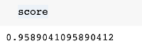
The model has given us excellent results. We will now use the model on an unseen data of a cancer patient to diagnose whether the cancer is benign or malignant at this stage.

25Inference on Unseen Data

Now let’s assume a real-world situation where a doctor gets the breast mass details of certain patients and he wants to find if it’s in a benign or malignant state of cancer. He can apply our model to get quite an accurate prediction for his patients.Let us load the five test cases in a list:

Now, we use KNN model on these cases:

testset = []
testset =  pd.DataFrame(testset) 
breast_mass_1_characteristics = [{'radius_mean': 21.1, 'perimeter_mean': 137.2, 'area_mean': 1404.0,
                        'concavity_mean': 0.1, 'concave points_mean': 0.0,'radius_worst': 29.1,
                        'perimeter_worst': 188.0, 'area_worst': 2615.0,'concavity_worst': 0.3,
                        'concave points_worst': 0.2}]
testset = testset.append(breast_mass_1_characteristics)
breast_mass_2_characteristics = [{'radius_mean': 14.5, 'perimeter_mean': 96.7, 'area_mean': 658.8,
                        'concavity_mean': 0.1, 'concave points_mean': 0.0,'radius_worst': 17.4,
                        'perimeter_worst': 124.1, 'area_worst': 943.2,'concavity_worst': 0.7,
                        'concave points_worst': 0.1}]
testset = testset.append(breast_mass_2_characteristics)
breast_mass_3_characteristics = [{'radius_mean': 15.3, 'perimeter_mean': 102.4, 'area_mean': 732.4,
                        'concavity_mean': 0.1, 'concave points_mean': 0.0,'radius_worst': 20.2,
                        'perimeter_worst': 149.3, 'area_worst': 1269.0,'concavity_worst': 0.6,
                        'concave points_worst': 0.2}]     
testset = testset.append(breast_mass_3_characteristics)
breast_mass_4_characteristics  = [{'radius_mean': 9.1, 'perimeter_mean': 59.2, 'area_mean': 260.9,
                        'concavity_mean': 0.0, 'concave points_mean': 0.0,'radius_worst': 10.0,
                        'perimeter_worst': 65.5, 'area_worst': 310.1,'concavity_worst': 0.1,
                        'concave points_worst': 0.05}]
testset = testset.append(breast_mass_4_characteristics )
breast_mass_5_characteristics  = [{'radius_mean': 11.5, 'perimeter_mean': 73.3, 'area_mean': 409.0,
                        'concavity_mean': 0.03, 'concave points_mean': 0.02,'radius_worst': 12.8,
                        'perimeter_worst': 81.8, 'area_worst': 506.2,'concavity_worst': 0.09,
                        'concave points_worst': 0.06}]
testset = testset.append(breast_mass_5_characteristics)


testset = zscore(testset)
testset = testset.values.tolist()

The output is as follows;

k_nearest_neighbors_model(dset, testset, 5)

We can see that the first three breast masses are most likely at the malignant stage and the last 2 at the begining stage. The doctor can now proceed with the treatment accordingly.

26Summary

In this tutorial, we built a working model of the KNN algorithm and implemented it in a real-world situation of detecting cancer type. You learned how to find the correlation between many features and then use feature engineering to reduce the number of features. We then developed the KNN model and applied it on the revised dataset to identify the cancer’s stage as benign or malignant. You then learned how to use this model on a real-life basis of few patient’s data (engineered) to detect the cancer stage.