01Introduction
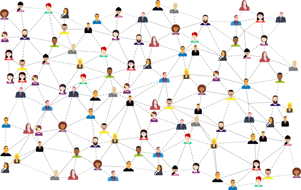
Ever wondered how Facebook suggests “People you may know” so accurately? Out of billions of registered users that Facebook has, it is a humongous task to search for the right connections. We analyze the entire network to find out features and see how two nodes (entities/people) are related, if they are friends or not?, if they have something in common?, how well are they connected to the rest of the network or a part of the network? and predict whether two nodes would connect with each other in future? And give us suggestions which we find in the “People you may know” section.
Understanding how Facebook does this analysis, can also help many large corporations to find similarity (attributes) between employees and get to know how much salary (attribute) a person should get based on salaries of other employees?, how fast an information will spread through the whole network if the information is provided to a certain node?, etc.. The study and analysis of networking will help a company grow and strengthen.
In this tutorial, I will show how to perform such an analysis. As this is an exhaustive topic, I am going to split this entire tutorial into three parts. In today’s part, I will cover the network visualization. By visualizing your company’s network, you will get a better idea about the geographical distribution of the entities and also several other attributes related to the employees
02Background
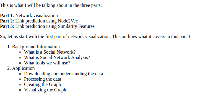
First, I will describe what a social network is. I will then explain to you the need of analyzing such networks and finally the tools available to you for performing such analysis.
05What tools we will use?
We use NetworkX library for network analysis. NetworkX is a python library used to study networks/graphs. It has many useful functions which can create, analyse, visualise, explore unique attributes and get an idea of the nodes and edges and the entire network overall. It can find transitivity (tendency of friends of friends to be friends and enemies of enemies to be enemies), reciprocity (if two nodes in an undirected graph can reach each other no matter the starting node), preferential attachment (popularity of a node in the network), degree centrality (the number of nodes a node connects to), betweenness centrality (the number of nodes that have to pass through a node to get to another node), and many more. We will calculate all the similarity measures using NetworkX.
Note - I’ll sometimes be saying edges and node pairs. Please understand these are the same, a particular node pair denotes the edge between them.
06Project
In this project, we will use the Facebook dataset provided by SNAP (Stanford Network Analysis Project). SNAP provides datasets for many social networking platforms. We can download the dataset from the SNAP site.
07Understanding Dataset
Here is the brief Information about the data:
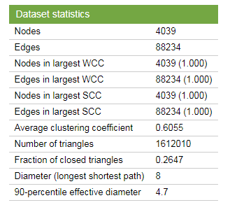
They provide the following files as part of the download.
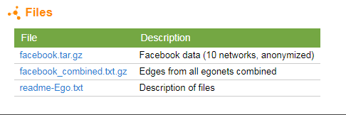
The facebook.tar.gz has 50 items, some of which are :
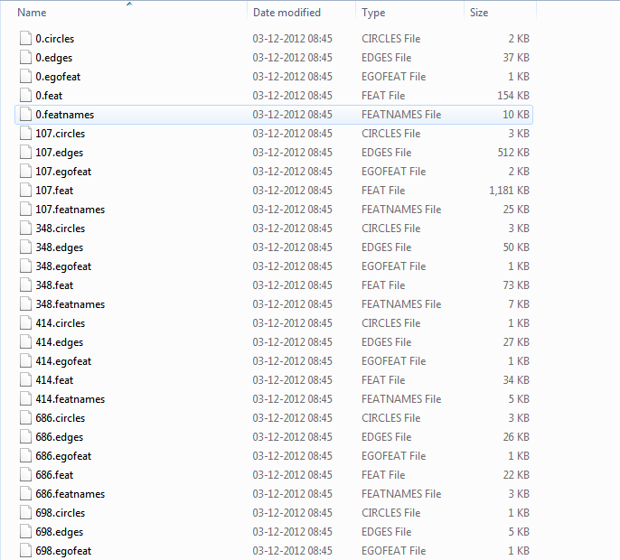
You can read the description on these files in the Standford's download site.
The nodeId.edges contain information of all the edges present in the network. The facebook_combined.txt contains the combined information on nodes and edges. What we require is nodeId.feat and nodeId.featnames files to add information at each node. The nodeId.featnames contains all the features/attributes in a particular set of nodes, and nodeId.feat is a file which contains every row as the set of nodes and every column as the node feature names provided in ‘nodeId.featnames’ file. Every column for a particular node is denoted by either ‘0’ or ‘1’, where ‘0’ means the node does not have the particular feature and ‘1’ means it has that feature.
08Import Libraries
Import the required libraries into your project:
import random
from tqdm import tqdm
import networkx as nx
import pandas as pd
import numpy as np
import matplotlib.pyplot as plt
import seaborn as sns
%matplotlib inline
from zipfile import ZipFile09Downloading Data
Download the data into your project using wget command and unzip its contents.
!wget https://github.com/abcom-mltutorials/Facebook-Social-Network-Analysis/archive/master.zip -P "/content"
ZipFile("/content/master.zip").extractall("/content/")
As mentioned earlier facebook_combined.txt contains the existing edges list. So we are going to import it and put it into pandas dataframe and name it ‘fb’.
fb = pd.read_csv('/content/Facebook-Social-Network-Analysis-master/facebook_combined.txt', delim_whitespace=True, names=['Source', 'Destination'])
fb
The output is as follows:
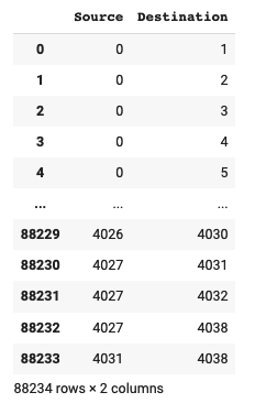
From the preceding screenshot, you can see that it connects the source node 4031 to the destination node 4038, while the source 4027 connects to three destinations 4031, 4032 and 4038.
Next, we will get the information on the features of each node.
10Extracting Feature Names
They store the feature names in the files with extension ‘.featnames’. The examples are ‘0.featnames’ and ‘107.featnames’; you will find these files in the facebook folder of your downloaded dataset. To examine the contents of one such file, let us read a file and print its contents:
with open('/content/Facebook-Social-Network-Analysis-master/facebook/0.featnames', 'r') as f:
       feature_names = f.readlines()
feature_names_df = pd.read_csv('/content/Facebook-Social-Network-Analysis-master/facebook/0.featnames', names=['Feature Names'])
feature_names_df
The output is as follows:
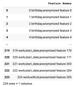
As you can see, there are 224 features; it represents each feature as number, name and type, with fields separated by a semicolon. All feature types are prefixed with “anonymized feature”.
You can also check how many unique features are there in this file (0.featnames) using the following code:
unique_features = []

for i in range(len(feature_names)):
 feature_names[i] = feature_names[i].split(' ', 1)[1]
 feature_names[i] = feature_names[i].rsplit(';' , 1)[0]
 unique_features.append(feature_names[i])

list(set(unique_features))
The output is as follows:
['work;employer;id',
 'locale',
 'education;school;id',
 'first_name',
 'location;id',
 'work;with;id',
 'last_name',
 'work;position;id',
 'languages;id',
 'education;degree;id',
 'hometown;id',
 'gender',
 'work;start_date',
 'education;concentration;id',
 'education;year;id',
 'birthday',
 'work;location;id',
 'education;classes;id',
 'education;with;id',
 'work;end_date',
 'education;type']
We need to extract only the name from the column value string and also need to merge the feature names from all .featnames files. For this, we will define a function:
def ExtractFeatureNames(path):
   with open(path, 'r') as f:
       feature_names = f.readlines()

   for i in range(len(feature_names)):
       feature_names[i] = feature_names[i].split(' ', 1)[1]
       feature_names[i] = feature_names[i].rsplit('
' , 1)[0]
       feature_names[i] = feature_names[i].rsplit(';' , 1)
       feature_names[i][1] = feature_names[i][1].rsplit(' ' , 1)[1]

   return feature_names
We will use the preceding function to get the merged list of all features
The .featnames files in our dataset have the following indexes:
l = ['0','107','348','414','686','698','1684','1912','3437','3980']These files contain information features for 4000+ nodes. The dataset creator has given different extensions, for example, the file with index 0 has extensions ‘0.feat’, ‘0.featnames’, ‘0.egofeat’, ‘0.circles’, ‘0.edges’. We will use only the file extensions ‘.feat’ and ‘.featnames’. We will extract only the location and education, school features for our dataset. We create the merged feature list using the following code:
for i in l:
   df = pd.read_csv('/content/Facebook-Social-Network-Analysis-master/facebook/'+i +'.feat',
                    delim_whitespace=True, names=pd.MultiIndex.from_tuples(ExtractFeatureNames('/content/Facebook-Social-Network-Analysis-master/facebook/'+i +'.featnames'))).T
node_features.append(df.loc[['location;id','education;school;id']])11Creating Dictionary of Nodes
Now, we will create a dataset containing nodes and their attributes (features). We will store the features along with the node and feature name into a nested dictionary where nodes will be the keys at the first level and feature names will be the keys at the second level. The feature values will be the dictionary values.
A node might have over one value for education school feature, we will use only the last/recent one. Also, we will ignore all the nodes having only one feature. The following code segment builds this nested dictionary.
node_attributes = {}
for i in node_features:
   a = {j : i[i[j] == 1][j].index.tolist()[-2:] for j in i.columns if len(i[i[j] == 1][j].index.tolist())>1 and
                                                                i[i[j] == 1][j].index.tolist()[-1][0] == 'location;id'}
   node_attributes.update(a)

#creating the nested dictionary
for k,v in node_attributes.items():
   node_attributes[k] = {i[0] : i[1] for i in node_attributes[k]}

#sorting the dictionary
node_attributes = {i[0]: i[1] for i in sorted(node_attributes.items())}
You may print a few records to see how the dictionary looks like:
list(node_attributes.items())[:10]The output is as follows:
[(2, {'education;school;id': '35', 'location;id': '135'}),
 (3, {'education;school;id': '50', 'location;id': '137'}),
 (7, {'education;school;id': '50', 'location;id': '137'}),
 (10, {'education;school;id': '50', 'location;id': '137'}),
 (13, {'education;school;id': '50', 'location;id': '137'}),
 (16, {'education;school;id': '50', 'location;id': '137'}),
 (17, {'education;school;id': '39', 'location;id': '129'}),
 (23, {'education;school;id': '47', 'location;id': '132'}),
 (24, {'education;school;id': '50', 'location;id': '132'}),
 (25, {'education;school;id': '50', 'location;id': '132'})]
We will now clean up our fb dataframe, which is the one we are going to use ultimately for network visualization.
12Dropping Unwanted Nodes from ‘fb’ Dataframe
As we have picked up only two features, location and education:school, the dictionary node_attributes might not have all the nodes present in the fb dataframe. Thus, we need to drop all the extra edges in fb.
#dropping the extra nodes from 'fb' that are not in 'node_attributes'
no_att_source = list(set([i for i in fb.Source]) - set(node_attributes.keys()))
no_att_dest = list(set([i for i in fb.Destination]) - set(node_attributes.keys()))

#finding indices of the above nodes in fb and dropping them
idx = []
for i in no_att_source:
   idx.extend(fb.index[fb.Source == i].tolist())

fb.drop(list(set(idx)), axis=0, inplace=True)

idx = []
for i in no_att_dest:
   idx.extend(fb.index[fb.Destination == i].tolist())

fb.drop(list(set(idx)), axis=0, inplace=True)13Create a List of Edges
We now create a list of edges. We create this list of node pair tuples from the fb dataframe:
existing_edges = [(fb.iloc[i,0],fb.iloc[i,1]) for i in range(fb.shape[0])]You may examine the contents of the list by printing a few records:
existing_edges[:5]The output is as follows:
[(2, 116), (2, 226), (2, 326), (3, 25), (3, 67)]From the output you can see that node 2 connects to three nodes 116, 226, and 326. Each of these nodes will have only two attributes, location and education. So, we now have a cleaned-up dataset ready for constructing a network graph.
14Creating the graph
Let’s create a graph, and add nodes and edges to it using NetworkX library.
G = nx.Graph()
for i in node_attributes.keys():
   G.add_node(i)
G.add_edges_from(existing_edges)
nx.set_node_attributes(G, node_attributes)
print(nx.info(G))
The output is as follows:
Name:
Type: Graph
Number of nodes: 1447
Number of edges: 18476
Average degree:  25.537
As you can see, we have 1447 nodes with 18376 edges. The average degree is 25.53. A degree shows the number of edges coming out of a node. Some of the nodes may have a small degree. To avoid cluttering in the visualization, we will drop all nodes with degree less than three.
deg = [i for i in G if G.degree(i) <3]
G.remove_nodes_from(deg)
print(nx.info(G))
The output is as follows:
Name:
Type: Graph
Number of nodes: 1295
Number of edges: 18321
Average degree:  28.2950
Finally, we will construct a new dataframe for plotting from the above graph.
fb = pd.DataFrame(data=list(G.edges()), columns=['Node 1', 'Node 2'])
fb.head()
The output is as follows:
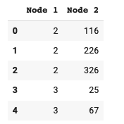
We are now all set for visualizing the network.
15Circular Layout
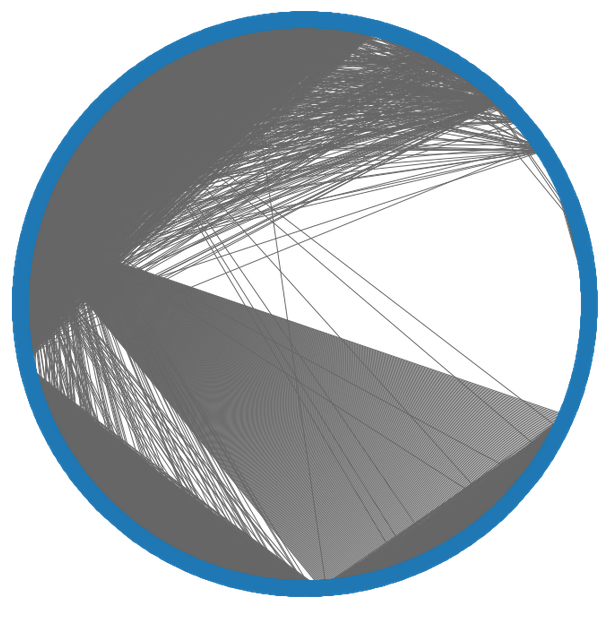
In circular layout, we place all nodes on the circumference of a circle. The connections from each node to other connected nodes are indicated by the lines connecting those points. This helps in showing the density distribution of the connections and the distance between the connecting nodes. We plot the layout using the following code:
plt.figure(figsize=(10,10))
pos = nx.circular_layout(G)
nx.draw_networkx(G, pos, with_labels=False, edge_color='.4')

plt.axis('off')
plt.tight_layout();
The output is as follows:
16Random Layout
In this layout, we place the nodes randomly within an area. We draw the connections between the nodes with lines. The layout will help in understanding the random distribution of the network. We plot the layout using following code:
plt.figure(figsize=(50,50))
pos = nx.random_layout(G)
nx.draw_networkx(G, pos, with_labels=False)

plt.axis('off')
plt.tight_layout();
The output is as follows:
17Spring Layout
The spring layout helps us understand if there are any isolated nodes in the graph. It also gives us clues on the number of connected components. The alpha parameter shows the color opacity for the node. We make the plot using following code:
plt.figure(figsize=(10,10))
nx.draw_networkx(G, alpha=0.7, with_labels=False)
plt.axis('off')
plt.tight_layout();
The output is as follows:
18Custom Layout
I will show you how to create customized visualizations. We will have node size changing with its degree. Thus, a node having many out connections will have a larger size. This will bring out the importance of such nodes. We will also use a different color for different locations. This will help us understand the locational distribution of the network. Likewise, you can customize the plot to bring out unique features in the network. The following code generates such a customized layout.
plt.figure(figsize=(30,30))

# node size is based on the degree of the node
node_size = [80*G.degree(v) for v in G]

# node color is based on the node attribute/feature value
node_color = [int(nx.get_node_attributes(G, 'location;id')[v]) for v in G]

colors=range(max(node_color))
cmap=plt.cm.Blues
vmin = min(colors)
vmax = max(colors)

# drawing graph with custom node size and color
# using spring layout
pos = nx.spring_layout(G)
nx.draw_networkx(G, pos, node_size=node_size,
                node_color=node_color, alpha=0.7,
                with_labels=False,
                edge_color='.4', cmap=cmap)

# getting the values according to attributes
# for the colorbar
sm = plt.cm.ScalarMappable(cmap=cmap,
                          norm=plt.Normalize(
                              vmin = vmin, vmax=vmax))
sm._A = []

plt.title('Size of a node depends on degree of the node
 Color of a node depends on the location attribute of a  the node', fontsize=40)
plt.axis('off')
plt.colorbar(sm)

#plotting annotations for different nodes
ax = plt.gca()
ax.annotate("Node 1", xy=pos.get(17), xytext=(0, 60),
           textcoords='offset points',
           arrowprops=dict(facecolor='black'))

ax1 = plt.gca()
ax1.annotate("Node 2", xy=pos.get(3280), xytext=(0, 60),
            textcoords='offset points',
            arrowprops=dict(facecolor='black'))

ax2 = plt.gca()
ax2.annotate("Node 3", xy=pos.get(1078), xytext=(0, 60), textcoords='offset points',
            arrowprops=dict(facecolor='black'))

plt.suptitle('

Degree of Node 1 (4) < Degree of Node 2 (31) < Degree of Node 3 (97)', fontsize=30)

plt.tight_layout();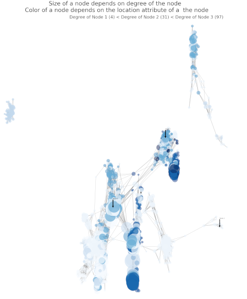
Observe the different node sizes that show its degree. The different shades of blue color point out the locational information.
From the above four charts, we can make a few following general comments on the network:
- The first two layouts tell us most of the nodes are well connected with each other.
- The third layout gives us an idea about the isolated nodes and also the number of connected components.
- The last custom layout gives us the idea on degrees of nodes, along with the distinction of their features.
Thus, by using different visualization techniques, you will analyze the network topology. Such analysis is very vital in making recommendations and for a massively enormous network like Facebook, such visualizations carry lots of weightage in network analysis.
19Saving Graph and Dataframe
We will also save the graph and the new ‘fb’ dataframe created here, which we will be using in the next part of the project.
nx.write_gpickle(G,'/content/Facebook-Social-Network-Analysis-Project-master/Graph.pickle')

fb.to_csv('Facebook-Social-Network-Analysis-Project-master/fb.csv', index=False)20Summary
In this tutorial, you learned how to extract the required data from the network files to create a graph and visualize it with various kinds of plots. The NetworkX library helps us in creating network graphs and to create visualizations. This is the first step in social network analysis.
The network data is mostly unorganized. You learned how to cleanse the data and organize it for constructing a graph. The data processing includes selecting desired features, dropping unwanted items (nodes/edges/features), converting data to an appropriate data structure, and so on. After pre-processing data, you learned to create graphs using the NetworkX library. You learned how to add nodes, edges and attributes/features to the graph. Graphs with isolated nodes or nodes with a low degree gives low/bad link prediction scores. You learned how to remove such nodes. Last, you learned how to create different network plots, including your own customized ones. That’s about it. So go on, and try out some of these methods in your next Social Network Analysis projects, and if you are new to this topic, try learning and replicating the above to get an idea. Good Luck!
In the next part (Part 2), I will show you how to do the network predictions using Node2Vec.

Arka Dyuti Kundu
Project idea, development and technical writing.
6 articles on ABCOM Education